Applied CAPM
Let’s study an example of calculating a CAPM \(\beta\) using real market data. Begin by loading the pandas_datareader module for importing data. We’ll also import the datetime module so that we can select stock prices over a given date range.
import pandas_datareader.data as web
from datetime import datetime
---------------------------------------------------------------------------
ModuleNotFoundError                       Traceback (most recent call last)
<ipython-input-1-3972f8269bfb> in <module>
----> 1 import pandas_datareader.data as web
      2 from datetime import datetime

ModuleNotFoundError: No module named 'pandas_datareader'
We’ll use AlphaVantage for stock prices. Load up the API key that we stored earlier.
import pickle
with open('../pickle_jar/av_key.p', 'rb') as f:
    api_key = pickle.load(f)
print(api_key[0:3])
VAS
The stock we’ll use for our study is AAPL. Let’s collect return data over 2015-2019.
start = datetime(2015, 1, 1)
end = datetime(2019, 12, 31)

aapl = web.DataReader('AAPL', 'av-daily-adjusted', start, end, api_key=api_key)
Print the head to see a snapshot of the data.
aapl.head()
| open | high | low | close | adjusted close | volume | dividend amount | split coefficient | |
|---|---|---|---|---|---|---|---|---|
| 2015-01-02 | 111.39 | 111.44 | 107.350 | 109.33 | 24.779987 | 53204626 | 0.0 | 1.0 |
| 2015-01-05 | 108.29 | 108.65 | 105.410 | 106.25 | 24.081896 | 64285491 | 0.0 | 1.0 |
| 2015-01-06 | 106.54 | 107.43 | 104.630 | 106.26 | 24.084162 | 65797116 | 0.0 | 1.0 |
| 2015-01-07 | 107.20 | 108.20 | 106.695 | 107.75 | 24.421875 | 40105934 | 0.0 | 1.0 |
| 2015-01-08 | 109.23 | 112.15 | 108.700 | 111.89 | 25.360219 | 59364547 | 0.0 | 1.0 |
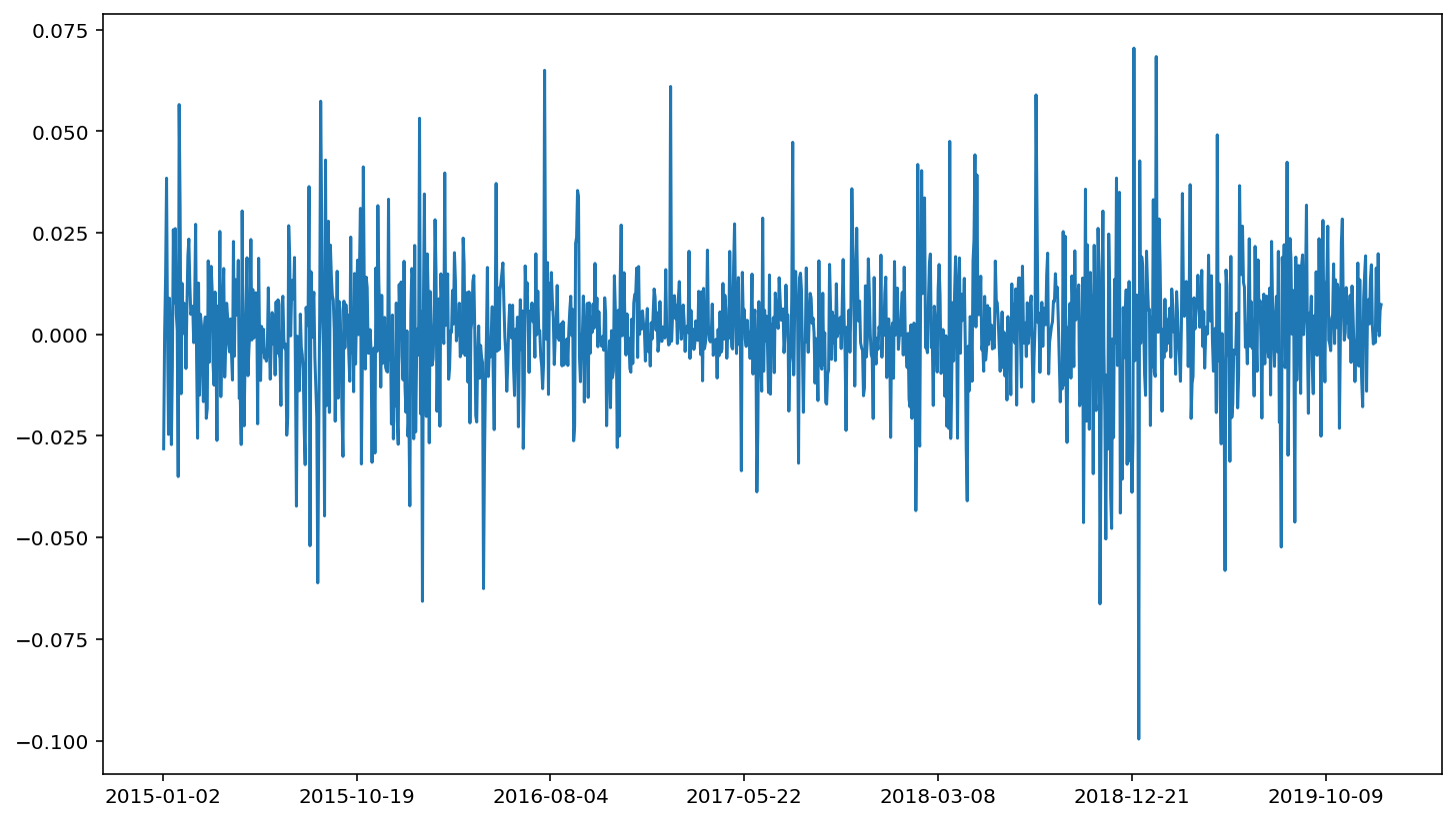
Create a column of stock returns using the adjusted close data.
aapl['ret'] = aapl['adjusted close'].pct_change()
aapl['ret'].plot()
<AxesSubplot:>
Now we need some market return data. The Fama-French data library has that available.
Note that Fama-French API calls via pandas_datareader return a dictionary of values, rather than a DataFrame.
ff = web.DataReader('F-F_Research_Data_Factors_daily', 'famafrench', start, end)
ff.keys()
dict_keys([0, 'DESCR'])
The 'DESCR' gives some details about the data while the 0 key stores the actual DataFrame.
print(ff['DESCR'])
F-F Research Data Factors daily
-------------------------------

This file was created by CMPT_ME_BEME_RETS_DAILY using the 202107 CRSP database. The Tbill return is the simple daily rate that, over the number of trading days in the month, compounds to 1-month TBill rate from Ibbotson and Associates Inc. Copyright 2021 Kenneth R. French

  0 : (1258 rows x 4 cols)
ffdf = ff[0]
ffdf.head()
| Mkt-RF | SMB | HML | RF | |
|---|---|---|---|---|
| Date | ||||
| 2015-01-02 | -0.12 | -0.62 | 0.08 | 0.0 |
| 2015-01-05 | -1.84 | 0.33 | -0.68 | 0.0 |
| 2015-01-06 | -1.04 | -0.78 | -0.31 | 0.0 |
| 2015-01-07 | 1.19 | 0.20 | -0.65 | 0.0 |
| 2015-01-08 | 1.81 | -0.11 | -0.28 | 0.0 |
One tricky issue is that, while the head printouts for the two DataFrames make the index items appear similar, they are not. Data from Fama-French returns an datetime variable as an index (which is more useful) whereas data from the AlphaVantage API call returns the index as a string.
print(aapl.index.dtype)
print(ffdf.index.dtype)
object
datetime64[ns]
We’ll want the index of the AlphaVantage data to be a datetime (to match the Fama-French data). To do this, we simply us the .to_datetime() function on the .index variable of the AlphaVantage DataFrame.
import pandas as pd
aapl.index = pd.to_datetime(aapl.index, format='%Y-%m-%d')
print(aapl.index.dtype)
datetime64[ns]
With both DataFrames using the same index, we can merge the two using the index value as the merge key. Thus, rather than using left_on and right_on to specify the merge variable, we specify left_index=True and right_index=True to tell Python that the merging variable will be the index.
df = aapl.merge(ffdf, left_index=True, right_index=True)
df.head()
| open | high | low | close | adjusted close | volume | dividend amount | split coefficient | ret | Mkt-RF | SMB | HML | RF | |
|---|---|---|---|---|---|---|---|---|---|---|---|---|---|
| 2015-01-02 | 111.39 | 111.44 | 107.350 | 109.33 | 24.779987 | 53204626 | 0.0 | 1.0 | NaN | -0.12 | -0.62 | 0.08 | 0.0 |
| 2015-01-05 | 108.29 | 108.65 | 105.410 | 106.25 | 24.081896 | 64285491 | 0.0 | 1.0 | -0.028172 | -1.84 | 0.33 | -0.68 | 0.0 |
| 2015-01-06 | 106.54 | 107.43 | 104.630 | 106.26 | 24.084162 | 65797116 | 0.0 | 1.0 | 0.000094 | -1.04 | -0.78 | -0.31 | 0.0 |
| 2015-01-07 | 107.20 | 108.20 | 106.695 | 107.75 | 24.421875 | 40105934 | 0.0 | 1.0 | 0.014022 | 1.19 | 0.20 | -0.65 | 0.0 |
| 2015-01-08 | 109.23 | 112.15 | 108.700 | 111.89 | 25.360219 | 59364547 | 0.0 | 1.0 | 0.038422 | 1.81 | -0.11 | -0.28 | 0.0 |
Remember that the \(y\) variable in a CAPM equation is the excess return of the stock. So, subtract the company’s return from the risk free rate.
df['eret'] = df['ret']*100 - df['RF']
We can now estimate a CAPM \(\beta\).
import statsmodels.formula.api as smf

mod = smf.ols('eret ~ Q("Mkt-RF")', data=df).fit()
print(mod.summary())
print(mod.params)
                            OLS Regression Results
==============================================================================
Dep. Variable:                   eret   R-squared:                       0.442
Model:                            OLS   Adj. R-squared:                  0.442
Method:                 Least Squares   F-statistic:                     995.8
Date:                Sun, 26 Sep 2021   Prob (F-statistic):          2.17e-161
Time:                        22:26:10   Log-Likelihood:                -1978.4
No. Observations:                1257   AIC:                             3961.
Df Residuals:                    1255   BIC:                             3971.
Df Model:                           1
Covariance Type:            nonrobust
===============================================================================
                  coef    std err          t      P>|t|      [0.025      0.975]
-------------------------------------------------------------------------------
Intercept       0.0417      0.033      1.264      0.206      -0.023       0.106
Q("Mkt-RF")     1.2009      0.038     31.556      0.000       1.126       1.276
==============================================================================
Omnibus:                      190.235   Durbin-Watson:                   1.884
Prob(Omnibus):                  0.000   Jarque-Bera (JB):             2298.267
Skew:                           0.241   Prob(JB):                         0.00
Kurtosis:                       9.607   Cond. No.                         1.16
==============================================================================

Notes:
[1] Standard Errors assume that the covariance matrix of the errors is correctly specified.
Intercept      0.041726
Q("Mkt-RF")    1.200855
dtype: float64
Putting this all together, we get the code below.
def get_beta(start, end, ticker):
    with open('../../pickle_jar/av_key.p', 'rb') as fout:
        api_key = pickle.load(fout)
    stock = web.DataReader(ticker, 'av-daily-adjusted', start, end, api_key=api_key)
    stock['ret'] = stock['adjusted close'].pct_change()*100
    ff = web.DataReader('F-F_Research_Data_Factors_daily', 'famafrench', start, end)[0]
    stock.index = pd.to_datetime(stock.index, format='%Y-%m-%d')
    df = stock.merge(ff, left_index=True, right_index=True)
    df['eret'] = df['ret'] - df['RF']
    mod = smf.ols('eret ~ Q("Mkt-RF")', data=df)
    res = mod.fit()
    print(res.summary())
    alpha, beta = res.params
    return beta

get_beta(start = datetime(2018,1,1), end = datetime(2019,12,31), ticker='GOOG')
                            OLS Regression Results
==============================================================================
Dep. Variable:                   eret   R-squared:                       0.587
Model:                            OLS   Adj. R-squared:                  0.587
Method:                 Least Squares   F-statistic:                     711.9
Date:                Sun, 26 Sep 2021   Prob (F-statistic):           3.49e-98
Time:                        22:31:28   Log-Likelihood:                -741.01
No. Observations:                 502   AIC:                             1486.
Df Residuals:                     500   BIC:                             1494.
Df Model:                           1
Covariance Type:            nonrobust
===============================================================================
                  coef    std err          t      P>|t|      [0.025      0.975]
-------------------------------------------------------------------------------
Intercept       0.0016      0.047      0.035      0.972      -0.091       0.095
Q("Mkt-RF")     1.3093      0.049     26.681      0.000       1.213       1.406
==============================================================================
Omnibus:                      147.463   Durbin-Watson:                   1.922
Prob(Omnibus):                  0.000   Jarque-Bera (JB):             7110.333
Skew:                           0.390   Prob(JB):                         0.00
Kurtosis:                      21.421   Cond. No.                         1.05
==============================================================================

Notes:
[1] Standard Errors assume that the covariance matrix of the errors is correctly specified.
1.3092647331440843