Regression
What function we use to estimate a relationship between \(y\) and the regressor(s) depends on the data that we have. As practice using multiple x-variables, let’s simulate a dataset that is generated by the following equation $\( y = 4 + 0.5 x + 3 x^2 + u \)$
The relationship between \(y\) and \(x\) in the above equation is said to be nonlinear in \(x\).
import pandas as pd
import numpy as np
import seaborn as sns
import statsmodels.formula.api as smf

np.random.seed(0)

df = pd.DataFrame(columns=['y', 'x', 'x2'])
df['x'] = np.random.normal(0, 1, 100)
df['x2'] = df['x'] ** 2
df['y'] = 4 + 0.5 * df['x'] + 3 * df['x2'] + np.random.normal(0, 0.5, 100)
df.head()
| y | x | x2 | |
|---|---|---|---|
| 0 | 15.159244 | 1.764052 | 3.111881 |
| 1 | 4.006576 | 0.400157 | 0.160126 |
| 2 | 6.727911 | 0.978738 | 0.957928 |
| 3 | 20.669952 | 2.240893 | 5.021602 |
| 4 | 14.810536 | 1.867558 | 3.487773 |
Note that to square column 'x' to produce 'x2', all we need to do is type df2['x'] ** 2 since ** is the command for exponentiation.
Next, plot a relationship between just y and x, assuming a linear fit.
sns.lmplot(x='x', y='y', data=df)
<seaborn.axisgrid.FacetGrid at 0x7fe0343631f0>
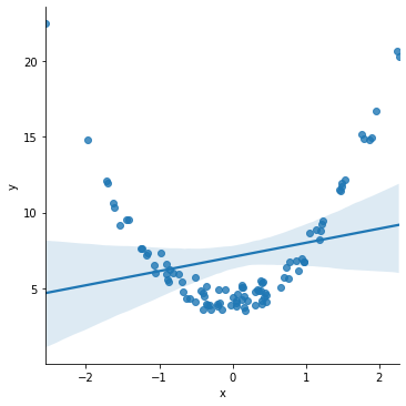
The estimated straight line gets things horribly wrong! The line is pretty far away from a lot of the actual data points.
The scatter plot of the data above makes clear that the data demonstrates a non-linear relationship.
What we ought do to is fit a line given by $\( \hat{y} = c + \hat{\beta}_1 x + \hat{\beta}_2 x^2 \)$
where there are two beta coefficients. One for \(x\), and one for \(x^2\).
model = smf.ols('y ~ x + x2', data=df).fit()
print(model.summary())
                            OLS Regression Results
==============================================================================
Dep. Variable:                      y   R-squared:                       0.983
Model:                            OLS   Adj. R-squared:                  0.983
Method:                 Least Squares   F-statistic:                     2885.
Date:                Mon, 06 Dec 2021   Prob (F-statistic):           3.91e-87
Time:                        12:06:14   Log-Likelihood:                -75.005
No. Observations:                 100   AIC:                             156.0
Df Residuals:                      97   BIC:                             163.8
Df Model:                           2
Covariance Type:            nonrobust
==============================================================================
                 coef    std err          t      P>|t|      [0.025      0.975]
------------------------------------------------------------------------------
Intercept      4.0714      0.066     61.584      0.000       3.940       4.203
x              0.5615      0.052     10.829      0.000       0.459       0.664
x2             2.9666      0.040     73.780      0.000       2.887       3.046
==============================================================================
Omnibus:                        7.876   Durbin-Watson:                   2.003
Prob(Omnibus):                  0.019   Jarque-Bera (JB):                3.580
Skew:                           0.188   Prob(JB):                        0.167
Kurtosis:                       2.152   Cond. No.                         2.47
==============================================================================

Notes:
[1] Standard Errors assume that the covariance matrix of the errors is correctly specified.
The variable model2 stores a lot of data. Beyond holding summary output for the performance of the regression (which we’ve accessed via the model2.summary() command), we can reference the estimated parameters directly via .params. For example:
print('Intercept: ', model.params['Intercept'])
print('beta for x:', model.params['x'])
print('beta for x2:', model.params['x2'])
Intercept:  4.071350754098632
beta for x: 0.5615154693913407
beta for x2: 2.9666242239334637
As an aside, the fact that we’re using square brackets to reference items inside of squared.params is a clue that the .params component of the variable squared was built using a dictionary-like structure.
One way to tell that the estimates of squared are better than the estimates of straight is to look at the R-squared value in the summary output. This measure takes a value between 0 and 1, with a score of 1 indicating perfect fit. For comparison purposes, consider the linear fit model below:
model_linear = smf.ols('y ~ x', data=df).fit()
print(model_linear.summary())
                            OLS Regression Results
==============================================================================
Dep. Variable:                      y   R-squared:                       0.056
Model:                            OLS   Adj. R-squared:                  0.046
Method:                 Least Squares   F-statistic:                     5.767
Date:                Mon, 06 Dec 2021   Prob (F-statistic):             0.0182
Time:                        12:06:14   Log-Likelihood:                -277.26
No. Observations:                 100   AIC:                             558.5
Df Residuals:                      98   BIC:                             563.7
Df Model:                           1
Covariance Type:            nonrobust
==============================================================================
                 coef    std err          t      P>|t|      [0.025      0.975]
------------------------------------------------------------------------------
Intercept      7.0734      0.392     18.054      0.000       6.296       7.851
x              0.9318      0.388      2.401      0.018       0.162       1.702
==============================================================================
Omnibus:                       49.717   Durbin-Watson:                   1.848
Prob(Omnibus):                  0.000   Jarque-Bera (JB):              128.463
Skew:                           1.877   Prob(JB):                     1.27e-28
Kurtosis:                       7.091   Cond. No.                         1.06
==============================================================================

Notes:
[1] Standard Errors assume that the covariance matrix of the errors is correctly specified.
The linear-fit model produced an R-squared of 0.056 while the quadratic-fit model yielded a R-squared of 0.983.
Another informative way to jude a modeled relationship is by plotting the residuals. The residuals are the “un-expected” part of the equation. For example, in the linear-fit model, the residual is defined as
$\(
\hat{u} := y - \hat{y} = y - \hat{c} - \hat{\beta} x
\)\(
and in the quadratic-fit model the residual, \)\hat{u}\(, is given by
\)\(
\hat{u} := y - \hat{y} = y- \hat{c} - \hat{\beta}_1 x - \hat{\beta}_2 x^2
\)$
Using the information in .params, we can calculate residuals.
df['resid'] = model.resid
df['resid_linear'] = model_linear.resid
Next, plot the two sets of residuals.
sns.scatterplot(x='x', y='resid_linear', data=df)
<AxesSubplot:xlabel='x', ylabel='resid_linear'>
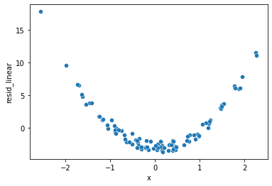
In the straight-line model, we can see that the errors have a noticeable pattern to them. This is an indication that a more complicated function of \(x\) would be a better description for the relationship between \(x\) and \(y\).
sns.scatterplot(x='x', y='resid', data=df)
<AxesSubplot:xlabel='x', ylabel='resid'>
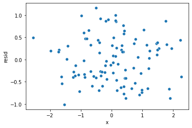
In comparison, the residuals from the squared model look more random. Additionally, they’re substantially smaller on average, with almost all residuals having an absolute value less than one. This indicates a much better fit than the straight-line model in which the residual values were often much larger.
Looking Beyond OLS
OLS works well when the \(y\) variable in our model is a linear combination of \(x\) variables. Note that the relationship between \(y\) and a given regressor may be nonlinear, as in the case of \(y\) being a function of \(x\) and \(x^2\). However, while we may say that \(y\) is a nonlinear function of \(x\) in this case, the variable \(y\) is still a linear function of \(x\) and \(x^2\). To clarify: $\( y = \alpha + \beta x + u \)\( is linear in \)x\(. Likewise: \)\( y = \alpha + \beta_1 x + \beta_2 x^2 + u \)\( is linear in \)x\( and \)x^2\(. In contrast, the function \)\( y = \frac{e^{\alpha + \beta x + u}}{1 + e^{\alpha + \beta x + u}} \)\( is *nonlinear*. This last equation may look terrifyingly unnatural, but it's actually very useful. Let's get a sense of what the equation looks like by plotting the function \)\( y = \frac{e^{x}}{1 + e^{x}}. \)$
np.random.seed(0)
curve = pd.DataFrame(columns=['x','y'])
curve['x'] = np.random.randint(low=-10, high=10, size=100)
curve['y'] = np.exp(curve['x']) / (1 + np.exp(curve['x']))
print(curve.head())
sns.lineplot(x='x', y='y', data=curve)
    x         y
0   2  0.880797
1   5  0.993307
2 -10  0.000045
3  -7  0.000911
4  -7  0.000911
<AxesSubplot:xlabel='x', ylabel='y'>
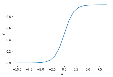
The function \(y = e^{x}/(1+e^{x})\) creates an S-curve with a lower bound of \(0\) and an upper bound of \(1\).
These bounds are useful in analytics. Often, our task is to estimate probabilities. For instance, what is the likelihood that a borrower defaults on their mortgage, the likelihood that a credit card transaction is fraudulent, or the likelihood that a company will violate its capital expenditure covenant on an outstanding loan? All of these questions require us to estimate a probability. The above function is useful because it considers a situation in which the \(y\) variable is necessarily between \(0\) and \(1\) (i.e. \(0\%\) probability and \(100\%\) probability).
Suppose that we instead took the curve data above and tried to fit it with linear regression.
sns.lmplot(x='x', y='y', data=curve)
<seaborn.axisgrid.FacetGrid at 0x7fe005c01ac0>
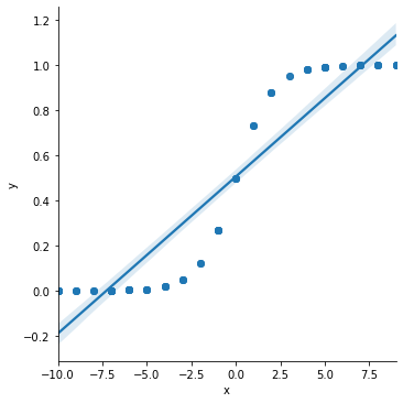
Note that in the above plot, there are estimated “probabilities” (the \(\hat{y}\) values) that are either lower than \(0\) or higher than \(1\). This is statistically impossible.
That fancy S-shaped function above is called the inverse logit function. That is because \(e^x / (1+e^x)\) is the inverse of the logit function given by \(log(x / (1-x)\). Just like we can invert the equation \(y = f(x)\) to get \(f^{-1}(y) = x\), the inverse of \(y = e^x / (1+e^x)\) is given by \(log(y / (1-y)) = x\).
When we model probabilities, the \(y\) variable will be either \(0\) or \(1\) for any observations. Observations where the event occurred are recorded with \(y=1\). For instance, in a dataset about mortgage default, those borrowers who default on their mortgage would have \(y=1\) and everyone else would have \(y=0\).
Suppose that we estimate a model given by $\( log\Big(\frac{y}{1-y}\Big) = \alpha + \beta x + u \)\(. Then, the estimated value \)\hat{\alpha} + \hat{\beta}x\( for a given observation would be \)log(\hat{y}/(1-\hat{y}))\(. This is what we refer to as the *log odds ratio*. The odds ratio is the probability that \)y\( equals \)1\( divided by the probability that \)y\( equals \)0\(; this is what \)\hat{y}/(1-\hat{y})\( tells us. Ultimately, our estimate for \)\hat{y}\( then tells us the likelihood that the true value for \)y\( is equal to \)1$.
This type of model is called a logistic regression model. Let’s simulate some data.
np.random.seed(0)
df2 = pd.DataFrame(columns=['x', 'y'])
df2['x'] = np.random.normal(2, 1, 1000)
df2['xb'] = -9 + 4 * df2['x']
df2['y'] = np.random.binomial(n=1, p= np.exp(df2['xb']) / (1+np.exp(df2['xb'])) )
df2.head()
| x | y | xb | |
|---|---|---|---|
| 0 | 3.764052 | 1 | 6.056209 |
| 1 | 2.400157 | 0 | 0.600629 |
| 2 | 2.978738 | 1 | 2.914952 |
| 3 | 4.240893 | 1 | 7.963573 |
| 4 | 3.867558 | 1 | 6.470232 |
Now try fitting a model using linear regression (ordinary least squares). When OLS is applied to a \(y\) variable that only takes value 0 or 1, the model is referred to as a linear probability model (LPM).
lpm = smf.ols('y ~ x', data=df2).fit()
print(lpm.summary())
                            OLS Regression Results
==============================================================================
Dep. Variable:                      y   R-squared:                       0.514
Model:                            OLS   Adj. R-squared:                  0.514
Method:                 Least Squares   F-statistic:                     1056.
Date:                Mon, 06 Dec 2021   Prob (F-statistic):          1.41e-158
Time:                        12:06:16   Log-Likelihood:                -346.17
No. Observations:                1000   AIC:                             696.3
Df Residuals:                     998   BIC:                             706.2
Df Model:                           1
Covariance Type:            nonrobust
==============================================================================
                 coef    std err          t      P>|t|      [0.025      0.975]
------------------------------------------------------------------------------
Intercept     -0.2928      0.024    -12.187      0.000      -0.340      -0.246
x              0.3564      0.011     32.493      0.000       0.335       0.378
==============================================================================
Omnibus:                      113.684   Durbin-Watson:                   2.045
Prob(Omnibus):                  0.000   Jarque-Bera (JB):               37.844
Skew:                           0.207   Prob(JB):                     6.06e-09
Kurtosis:                       2.142   Cond. No.                         5.70
==============================================================================

Notes:
[1] Standard Errors assume that the covariance matrix of the errors is correctly specified.
Now fit the model using logistic regression.
logit = smf.logit('y ~ x', data=df2).fit()
print(logit.summary())
Optimization terminated successfully.
         Current function value: 0.292801
         Iterations 8
                           Logit Regression Results
==============================================================================
Dep. Variable:                      y   No. Observations:                 1000
Model:                          Logit   Df Residuals:                      998
Method:                           MLE   Df Model:                            1
Date:                Mon, 06 Dec 2021   Pseudo R-squ.:                  0.5660
Time:                        12:06:16   Log-Likelihood:                -292.80
converged:                       True   LL-Null:                       -674.60
Covariance Type:            nonrobust   LLR p-value:                4.432e-168
==============================================================================
                 coef    std err          z      P>|z|      [0.025      0.975]
------------------------------------------------------------------------------
Intercept     -8.5975      0.567    -15.154      0.000      -9.709      -7.486
x              3.8987      0.259     15.062      0.000       3.391       4.406
==============================================================================
The estimated parameters (intercept and \(\beta\) coefficient) are much closer to their true value using logistic regression. While popular, linear probability models do not often give meaningful estimates. This is especially true when outcomes are rare (meaning most \(y\) values are either 0 or 1, and there is not a relatively even balance between the two).