American Community Survey
The American Community Survey(ACS) is the largest survey conducted by the U.S. Census Bureau. It collects basic demographic information about people living across the United States.
The survey is conducted every year, and, due to processing time, releases with a lag. For instance, the 2018 survey data is released in the latter part of 2019. The ACS data is relased not only in one-year estimates (e.g. 2018 survey data) but also in five-year estimates (e.g. 2014-2018 survey data). The one-year estimates are, naturally, more recent. However, five-year estimates may be necessary in some applications. The Census Bureau does not release survey information for small populations, due to anonymity concerns, every year. Rather, some information is available exclusively in the five-year survey data (which averages over a five year period).
A brief overview of the data available through the ACS is available here. Note that the ACS data includes things like age, marital status, income, employment status, and educational attainment.
The full list of ACS data is available here.
Register for an API key with the U.S. Census Bureau here. This step is required to continue with the lecture notes!
To keep my key secret, I’ve pickled the string that stores it, and will re-load it here.
import pickle
with open('../pickle_jar/census.p', 'rb') as f:
    api_key = pickle.load(f)
print(api_key[0:5])
6efdf
The formula to get data from the ACS is:
'https://api.census.gov/data/'
+ <year>
+ '/acs/acs1?get=NAME,'
+ <variable name>
+ '&for='
+ <geography>
+ ':*&key='
+ <API key>
For instance, to get median household income (which has <variable name> = B19013_001E) for <year> = 2010 over the entire U.S. (<geography> = us), we would use the string
'https://api.census.gov/data/' + '2010' + '/acs/acs1?get=NAME,' + 'B19013_001E' + '&for=' + 'us' + ':*&key=' + api_key
as our URL. An example request is shown below:
NOTE: Starting Fall 2021, we began to encounter issues with students receiving API keys from the Census Bureau that do not appear to work correctly. If the code below does not work for you, please replace it with the following Python code:
import requests
r = requests.get(‘https://raw.githubusercontent.com/learning-fintech/data/main/census/census1.json’).json()
print(r)
import requests
r = requests.get('https://api.census.gov/data/2018/acs/acs1?get=NAME,B19013_001E&for=us:*&key=' + api_key).json()
print(r)
[['NAME', 'B19013_001E', 'us'], ['United States', '61937', '1']]
Likewise, to get data for every county in the country, we would replace us with county following the for= piece of the string. This will return data on many counties. Instead of printing them all, below, we’ve printed just a sample, as well as the total number of counties for which median household income data is available via ACS.
NOTE: Starting Fall 2021, we began to encounter issues with students receiving API keys from the Census Bureau that do not appear to work correctly. If the code below does not work for you, please replace it with the following Python code:
import requests
r = requests.get(‘https://raw.githubusercontent.com/learning-fintech/data/main/census/census2.json’).json()
print(r)
r = requests.get('https://api.census.gov/data/2018/acs/acs1?get=NAME,B19013_001E&for=county:*&key=' + api_key).json()
print(r[0:10])
[['NAME', 'B19013_001E', 'state', 'county'], ['Baldwin County, Alabama', '56813', '01', '003'], ['Calhoun County, Alabama', '45818', '01', '015'], ['Cullman County, Alabama', '44612', '01', '043'], ['DeKalb County, Alabama', '36998', '01', '049'], ['Elmore County, Alabama', '60796', '01', '051'], ['Etowah County, Alabama', '45868', '01', '055'], ['Houston County, Alabama', '48105', '01', '069'], ['Jefferson County, Alabama', '55206', '01', '073'], ['Lauderdale County, Alabama', '49014', '01', '077']]
Note that the first item in this list is:
r[0]
['NAME', 'B19013_001E', 'state', 'county']
which is simply a set of headers. That is, for each additional item in the list, the data in position 0 is the county name and the data in position 1 corresponds to the value for the variable B19013_001E. The numbers in positions 2 and 3 are the county’s FIPS code. States have 2-digit FIPS codes, and counties have 3-digit FIPS codes. If we put the state code and county code together to a 5-digit number (state code then county code), we have a unique identifier for the county. This FIPS code is used by many different data providers.
Recall that we can remove an element from a list with the .pop() function. For instance, let’s remove the first element of our requested ACS data (the set of headers).
headers = r.pop(0) # delete item 0 from the list and simultaneously store it in the variable "headers"
Do not run the above line of code multiple times! Python will continue popping out elements of your list.
The value for headers is thus:
print(headers)
['NAME', 'B19013_001E', 'state', 'county']
as expected. Now, the requested ACS data no longer has that element. Rather, what is left is
print(r[0:3])
[['Baldwin County, Alabama', '56813', '01', '003'], ['Calhoun County, Alabama', '45818', '01', '015'], ['Cullman County, Alabama', '44612', '01', '043']]
simply data. This is useful, because we can not store all of the data we have in a DataFrame. The command to do this is pd.DataFrame(). This function takes two arguments. First, Python expects to receive a list of lists. This list of lists should correspond to the data that we want to store. The list of list is a list of rows of data, where each row may be a list of multiple values (multiple columns). The second argument is a list of column names.
import pandas as pd
census = pd.DataFrame(r, columns=headers)
census.head()
| NAME | B19013_001E | state | county | |
|---|---|---|---|---|
| 0 | Baldwin County, Alabama | 56813 | 01 | 003 |
| 1 | Calhoun County, Alabama | 45818 | 01 | 015 |
| 2 | Cullman County, Alabama | 44612 | 01 | 043 |
| 3 | DeKalb County, Alabama | 36998 | 01 | 049 |
| 4 | Elmore County, Alabama | 60796 | 01 | 051 |
Note that the state and county variables display with leading zeroes. That is, a number 1 is printed out at 01. This is a telltale sign that these columns are strings.
We will want these columns to be integers. The reason why will become apparent once we load another dataset. However, it’s convenient for us to convert the data type now. Remember that we could do int('01') to convert one string to one integer. In pandas, we can use the .astype() function on a column of string data to convert all rows of that column.
census['state'] = census['state'].astype(int)
census['county'] = census['county'].astype(int)
We can check the variable types formally with the .dtypes command.
census.dtypes
NAME           object
B19013_001E    object
state           int64
county          int64
dtype: object
Oh no! It looks like B19013_001E (the Census variable for median household income) is also a string (which pandas lumps into a group called object). So, we’ll want to convert median household income to an integer as well. This will allow us to use it in a regression later.
census['B19013_001E'] = census['B19013_001E'].astype(int)
Zillow Home Values
County median incomes give a sense of the economic well-being of a geographic area. Suppose that our interest is in how home prices (for most households, the most valuable asset that the household owns), correlates with income.
Housing data is available from Zillow here.
The URL for data on all home prices in a county (single-family residential and condos) is something like 'https://files.zillowstatic.com/research/public_csvs/zhvi/County_zhvi_uc_sfrcondo_tier_0.33_0.67_sm_sa_month.csv'. You can find these links from the page linked above. Pandas can read online csv files directly in to Python. The precise link from Zillow changes as they update their data, and old links can die over time. To avoid link rot, a copy of the Zillow data to use is made available at:
zhvi = pd.read_csv('https://raw.githubusercontent.com/learning-fintech/data/main/zhvi/County_zhvi_uc_sfrcondo_tier_0.33_0.67_sm_sa_month.csv')
The .shape property of a Pandas DataFrame reports the numbers of rows and columns.
zhvi.shape
(2822, 269)
There are a lot of columns on this file! Recall that the .columns property of a DataFrame returns a list of columns. Recall too that we can subset a list named x to items m through n via x[m:n]. Thus, print out only the first 20 columns of the DataFrame below (to get a sense of what’s included on this DataFrame).
zhvi.columns[0:20]
Index(['RegionID', 'SizeRank', 'RegionName', 'RegionType', 'StateName',
       'State', 'Metro', 'StateCodeFIPS', 'MunicipalCodeFIPS', '2000-01-31',
       '2000-02-29', '2000-03-31', '2000-04-30', '2000-05-31', '2000-06-30',
       '2000-07-31', '2000-08-31', '2000-09-30', '2000-10-31', '2000-11-30'],
      dtype='object')
Likewise, the last n items of list x are accessible via x[-n:].
zhvi.columns[-20:]
Index(['2020-01-31', '2020-02-29', '2020-03-31', '2020-04-30', '2020-05-31',
       '2020-06-30', '2020-07-31', '2020-08-31', '2020-09-30', '2020-10-31',
       '2020-11-30', '2020-12-31', '2021-01-31', '2021-02-28', '2021-03-31',
       '2021-04-30', '2021-05-31', '2021-06-30', '2021-07-31', '2021-08-31'],
      dtype='object')
Given what we observe about the data, define a list of column names to keep. All other columns outside of this list will be removed.
keep_list = [col for col in zhvi.columns[0:9]] + ['2018-12-31']
print(keep_list)
['RegionID', 'SizeRank', 'RegionName', 'RegionType', 'StateName', 'State', 'Metro', 'StateCodeFIPS', 'MunicipalCodeFIPS', '2018-12-31']
Tell Python to only keep those columns.
zhvi = zhvi[keep_list]
To inspect the data, print out a head.
zhvi.head()
| RegionID | SizeRank | RegionName | RegionType | StateName | State | Metro | StateCodeFIPS | MunicipalCodeFIPS | 2018-12-31 | |
|---|---|---|---|---|---|---|---|---|---|---|
| 0 | 3101 | 0 | Los Angeles County | County | CA | CA | Los Angeles-Long Beach-Anaheim | 6 | 37 | 633036.0 |
| 1 | 139 | 1 | Cook County | County | IL | IL | Chicago-Naperville-Elgin | 17 | 31 | 256785.0 |
| 2 | 1090 | 2 | Harris County | County | TX | TX | Houston-The Woodlands-Sugar Land | 48 | 201 | 197363.0 |
| 3 | 2402 | 3 | Maricopa County | County | AZ | AZ | Phoenix-Mesa-Scottsdale | 4 | 13 | 273091.0 |
| 4 | 2841 | 4 | San Diego County | County | CA | CA | San Diego-Carlsbad | 6 | 73 | 593304.0 |
We will combine datasets using state and county codes. Note that in the Zillow data, state and county codes were imported as numbers. We can check that below. The columns of interest are StateCodeFIPS and MunicipalCodeFIPS.
zhvi.dtypes
RegionID               int64
SizeRank               int64
RegionName            object
RegionType            object
StateName             object
State                 object
Metro                 object
StateCodeFIPS          int64
MunicipalCodeFIPS      int64
2018-12-31           float64
dtype: object
Now we can merge. The format for merging df1 and df2 is to use df1.merge(df2, left_on=, right_on=). The left_on and right_on specify variables on the left (df1) and right (df2) datasets that should link the datasets together. Note that df1 is the left dataset because it appears before .merge, whereas df2 is the right data because it appears after .merge. It is also possible to use df2.merge(df1, left_on=, right_on=). In this scenario, the lists passed to left_on and right_on would flip from the earlier usage (since now df2 is the left dataset).
df = zhvi.merge(census, left_on=['StateCodeFIPS', 'MunicipalCodeFIPS'], right_on=['state', 'county'])
Print the head to see a snapshot of the data.
df.head()
| RegionID | SizeRank | RegionName | RegionType | StateName | State | Metro | StateCodeFIPS | MunicipalCodeFIPS | 2018-12-31 | NAME | B19013_001E | state | county | |
|---|---|---|---|---|---|---|---|---|---|---|---|---|---|---|
| 0 | 3101 | 0 | Los Angeles County | County | CA | CA | Los Angeles-Long Beach-Anaheim | 6 | 37 | 633036.0 | Los Angeles County, California | 68093 | 6 | 37 |
| 1 | 139 | 1 | Cook County | County | IL | IL | Chicago-Naperville-Elgin | 17 | 31 | 256785.0 | Cook County, Illinois | 63353 | 17 | 31 |
| 2 | 1090 | 2 | Harris County | County | TX | TX | Houston-The Woodlands-Sugar Land | 48 | 201 | 197363.0 | Harris County, Texas | 60232 | 48 | 201 |
| 3 | 2402 | 3 | Maricopa County | County | AZ | AZ | Phoenix-Mesa-Scottsdale | 4 | 13 | 273091.0 | Maricopa County, Arizona | 65252 | 4 | 13 |
| 4 | 2841 | 4 | San Diego County | County | CA | CA | San Diego-Carlsbad | 6 | 73 | 593304.0 | San Diego County, California | 79079 | 6 | 73 |
This merged dataset has both county median income and an index of home values in the area.
We want to study median income and hope prices, but, let’s be honest, the variable name B19013_001E is awful. It’s tedious to type out, and it’s not particularly easy to remember. The pandas module has a tool to rename columns, so let’s use that. The syntax is <dataframe name>.rename(columns={<old name>: <new name>}). This does not update the dataset to use the new column name. Rather, the .rename() function returns a copy of the dataset with the new name. So, you need to do
<dataframe name> = <dataframe name>.rename(columns={<old name>: <new name>})
to have the change take effect.
df = df.rename(columns={'B19013_001E': 'med_inc', '2018-12-31': 'home_value'})
Are income and home prices correlated? We can quickly visualize the question with seaborn.
import seaborn as sns
sns.lmplot(x='med_inc', y='home_value', data=df)
<seaborn.axisgrid.FacetGrid at 0x7f7790d79e80>
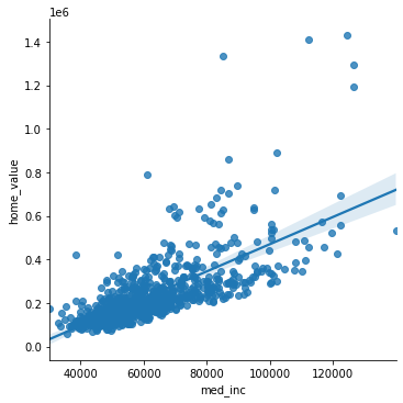
There do appear to be some outliers here. To check, try a boxplot.
sns.boxplot(x=df['home_value'])
<AxesSubplot:xlabel='home_value'>
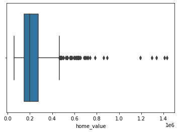
Additionally, print out a description of the home value index data.
df['home_value'].describe()
count    8.180000e+02
mean     2.349062e+05
std      1.489023e+05
min      5.683700e+04
25%      1.465330e+05
50%      1.970455e+05
75%      2.733452e+05
max      1.431949e+06
Name: home_value, dtype: float64
One method of removing outliers is to ignore (i.e. delete) the data that is “far out” on the boxplot (i.e., well beyond the whiskers).
The numpy module has a nanquantile() function to retrieve the 25th and 75th percentiles, as reported above in the summary statistics.
import numpy as np
quantiles = np.nanquantile(df['home_value'], q=[.25, .75])
print(quantiles)
[146533. 273345.25]
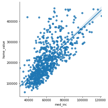
The interquartile range (IQR) is defined as the difference between the 75th and 25th percentiles of data. One reasonable way to remove outliers is to eliminate observations that exceed the 75th percentile by more than 1.5*IQR or are less than the 25th percentile by more than 1.5*IQR.
iqr = quantiles[1] - quantiles[0]
minidf = df[ (df['home_value'] < quantiles[1]+1.5*iqr) & (df['home_value'] > quantiles[0]-1.5*iqr) ].copy()
sns.lmplot(x='med_inc', y='home_value', data=minidf)
<seaborn.axisgrid.FacetGrid at 0x7f778b6c0f40>
import statsmodels.formula.api as smf

reg = smf.ols(formula='home_value ~ med_inc', data=minidf)
res = reg.fit(cov_type='HC3')
print(res.summary())
                            OLS Regression Results
==============================================================================
Dep. Variable:             home_value   R-squared:                       0.501
Model:                            OLS   Adj. R-squared:                  0.500
Method:                 Least Squares   F-statistic:                     898.7
Date:                Mon, 06 Dec 2021   Prob (F-statistic):          2.71e-131
Time:                        12:06:12   Log-Likelihood:                -9537.5
No. Observations:                 769   AIC:                         1.908e+04
Df Residuals:                     767   BIC:                         1.909e+04
Df Model:                           1
Covariance Type:                  HC3
==============================================================================
                 coef    std err          z      P>|z|      [0.025      0.975]
------------------------------------------------------------------------------
Intercept  -3.785e+04   8162.170     -4.637      0.000   -5.38e+04   -2.18e+04
med_inc        4.0613      0.135     29.978      0.000       3.796       4.327
==============================================================================
Omnibus:                      180.637   Durbin-Watson:                   1.939
Prob(Omnibus):                  0.000   Jarque-Bera (JB):              365.267
Skew:                           1.323   Prob(JB):                     4.82e-80
Kurtosis:                       5.097   Cond. No.                     2.65e+05
==============================================================================

Notes:
[1] Standard Errors are heteroscedasticity robust (HC3)
[2] The condition number is large, 2.65e+05. This might indicate that there are
strong multicollinearity or other numerical problems.