The pandas_datareader Module
In previous parts of this chapter, we discussed APIs. We use APIs to interface with data on a web server and bring that data in to Python.
In this section, we make use of the pandas_datareader module. This is a module that provides a set of API features to Python in such a way that the data is directly loaded in to a pandas DataFrame format. The pandas_datareader module actually used to be part of the pandas module, but it was spun off in to its own separate module.
import pandas_datareader.data as web
---------------------------------------------------------------------------
ModuleNotFoundError                       Traceback (most recent call last)
<ipython-input-1-bc32bb8bec34> in <module>
----> 1 import pandas_datareader.data as web

ModuleNotFoundError: No module named 'pandas_datareader'
Let’s start with an example provided in the module’s documentation.
from datetime import datetime

start = datetime(2005, 1, 1)
end = datetime(2019, 12, 31)

gdp = web.DataReader('GDP', 'fred', start, end)

gdp.head()
| GDP | |
|---|---|
| DATE | |
| 2005-01-01 | 12767.286 |
| 2005-04-01 | 12922.656 |
| 2005-07-01 | 13142.642 |
| 2005-10-01 | 13324.204 |
| 2006-01-01 | 13599.160 |
The above yields a data series of GDP values, listed at a quarterly frequency. Note that the DATE listed in the above DataFrame is not a column of data, it contains the labels for the rows. Remember, label names are bold-faced, so the name 2010-01-01 being in bold tells you that this is a row label, just like the name GDP in bold tells you that this is a column label.
Above, we accessed data from the 'fred' data provider. The FRED (Federal Reserve Economic Data) is an important provider of macroeconomic data, like measurement of gross domestic product.
Note that we can collect multiple data series from FRED simultaneously by requesting a list of data series in the first argument to the DataReader() function, as shown below.
inflation = web.DataReader(['CPIAUCSL', 'CPILFESL'], 'fred', start, end)

inflation.head()
| CPIAUCSL | CPILFESL | |
|---|---|---|
| DATE | ||
| 2005-01-01 | 191.6 | 199.0 |
| 2005-02-01 | 192.4 | 199.4 |
| 2005-03-01 | 193.1 | 200.1 |
| 2005-04-01 | 193.7 | 200.2 |
| 2005-05-01 | 193.6 | 200.5 |
We see two columns of data printed above, corresponding to the two data series names that were requested. But how are these series names chosen? The name 'CPIAUCSL', for instance, is not an intuitive name for “inflation.” And if 'CPIAUCSL' and 'CPILFESL' are both data about inflation, what makes them different?
If you search for a data series name on the FRED website, it will take you to the data series. Thus, we can easily find that:
CPIAUCSL is the consumer price index for urban consumers
CPILFESL is the consumer price index for urban consumers, excluding food and energy costs
Data on FRED are organized by category,and consumer price indexes are one such category.
We could get the consumer price index for just alcohol using the data series 'CUSR0000SAF116'.
alcohol = web.DataReader('CUSR0000SAF116', 'fred', start, end)

alcohol.head()
| CUSR0000SAF116 | |
|---|---|
| DATE | |
| 2005-01-01 | 194.6 |
| 2005-02-01 | 195.0 |
| 2005-03-01 | 195.2 |
| 2005-04-01 | 195.5 |
| 2005-05-01 | 195.3 |
Price indices are interesting, but let’s focus on some financial time series.
data_list = ['DGS1MO', 'DGS3MO', 'DGS6MO', 'DGS1', 'DGS2', 'DGS5', 'DGS7', 'DGS10', 'DGS30']

ts = web.DataReader(data_list, 'fred', start, end)

ts.head()
| DGS1MO | DGS3MO | DGS6MO | DGS1 | DGS2 | DGS5 | DGS7 | DGS10 | DGS30 | |
|---|---|---|---|---|---|---|---|---|---|
| DATE | |||||||||
| 2005-01-03 | 1.99 | 2.32 | 2.63 | 2.79 | 3.10 | 3.64 | 3.94 | 4.23 | 4.85 |
| 2005-01-04 | 2.05 | 2.33 | 2.63 | 2.82 | 3.20 | 3.72 | 4.02 | 4.29 | 4.91 |
| 2005-01-05 | 2.04 | 2.33 | 2.63 | 2.83 | 3.22 | 3.73 | 4.02 | 4.29 | 4.88 |
| 2005-01-06 | 2.04 | 2.31 | 2.63 | 2.82 | 3.18 | 3.71 | 4.01 | 4.29 | 4.89 |
| 2005-01-07 | 2.03 | 2.32 | 2.63 | 2.82 | 3.20 | 3.73 | 4.03 | 4.29 | 4.88 |
The data returned provides the term structure of interest rates. Interest rates on treasuries of varying maturities are collected.
It’s time to treat these row labels a bit more formally.
Recall that column labels can be accessed like so.
ts.columns
Index(['DGS1MO', 'DGS3MO', 'DGS6MO', 'DGS1', 'DGS2', 'DGS5', 'DGS7', 'DGS10',
       'DGS30'],
      dtype='object')
The columns of a DataFrame are referred to as, quite intuitively, columns!
The row labels are a bit different, they are typically referred to as the index of the DataFrame. The list of row labels is thus accessible via:
ts.index
DatetimeIndex(['2005-01-03', '2005-01-04', '2005-01-05', '2005-01-06',
               '2005-01-07', '2005-01-10', '2005-01-11', '2005-01-12',
               '2005-01-13', '2005-01-14',
               ...
               '2019-12-18', '2019-12-19', '2019-12-20', '2019-12-23',
               '2019-12-24', '2019-12-25', '2019-12-26', '2019-12-27',
               '2019-12-30', '2019-12-31'],
              dtype='datetime64[ns]', name='DATE', length=3912, freq=None)
It is at this point that use of .loc becomes interesting and useful, rather than simply an academic point about the structure of DataFrames. For instance, to look up the term structure of interest rates on June 7, 2019, we would enter:
ts.loc['2019-06-07']
DGS1MO    2.30
DGS3MO    2.28
DGS6MO    2.15
DGS1      1.97
DGS2      1.85
DGS5      1.85
DGS7      1.97
DGS10     2.09
DGS30     2.57
Name: 2019-06-07 00:00:00, dtype: float64
It’s helpful to have an index because it lets us label the data in two dimensions at once. The column label will tell us the name of the data series (e.g. 'DGS1', which is the yield on a set of 1 year constant maturity U.S. treasuries) and the row index will tell us the time at which that data is observed.
In earlier parts of this book, the row index was boring. Unless explicitly given a list of row labels to use for the index, Python will assign the row index to be the row number. For example:
import pandas as pd
import numpy as np
np.random.seed(0)
df = pd.DataFrame(columns=['x'])
df['x'] = np.random.normal(0, 1, 10)
df.head()
| x | |
|---|---|
| 0 | 1.764052 |
| 1 | 0.400157 |
| 2 | 0.978738 |
| 3 | 2.240893 |
| 4 | 1.867558 |
Note that the data returned from pandas_datareader is indexed in a very convenient way. Along with using ts.loc['2019-06-07'], we can get slices of the data like so:
ts.loc['2005-01-03':'2005-01-10']
| DGS1MO | DGS3MO | DGS6MO | DGS1 | DGS2 | DGS5 | DGS7 | DGS10 | DGS30 | |
|---|---|---|---|---|---|---|---|---|---|
| DATE | |||||||||
| 2005-01-03 | 1.99 | 2.32 | 2.63 | 2.79 | 3.10 | 3.64 | 3.94 | 4.23 | 4.85 |
| 2005-01-04 | 2.05 | 2.33 | 2.63 | 2.82 | 3.20 | 3.72 | 4.02 | 4.29 | 4.91 |
| 2005-01-05 | 2.04 | 2.33 | 2.63 | 2.83 | 3.22 | 3.73 | 4.02 | 4.29 | 4.88 |
| 2005-01-06 | 2.04 | 2.31 | 2.63 | 2.82 | 3.18 | 3.71 | 4.01 | 4.29 | 4.89 |
| 2005-01-07 | 2.03 | 2.32 | 2.63 | 2.82 | 3.20 | 3.73 | 4.03 | 4.29 | 4.88 |
| 2005-01-10 | 2.07 | 2.36 | 2.67 | 2.86 | 3.23 | 3.75 | 4.03 | 4.29 | 4.86 |
There are two important things to notice about index slicing here (slicing is another term for getting a subset of data).
First, the slice ends at the endpoint, not just before it. This breaks from normal Python convention. For instance, range(0:10) will give you the numbers 0 through 9, not the numbers 0 through 10. When slicing by index, the last row label you include is the last row you get. As another example:
df.loc[1:2]
| x | |
|---|---|
| 1 | 0.400157 |
| 2 | 0.978738 |
Second, the data exists for Jan. 3-7 and Jan. 10, but not for Jan. 8-9. Why? Because Jan. 8-9 was a weekend.
We can shift date indexes around quite easily via .shift(). This will come in handy in many applications.
ts.head(6)
| DGS1MO | DGS3MO | DGS6MO | DGS1 | DGS2 | DGS5 | DGS7 | DGS10 | DGS30 | |
|---|---|---|---|---|---|---|---|---|---|
| DATE | |||||||||
| 2005-01-03 | 1.99 | 2.32 | 2.63 | 2.79 | 3.10 | 3.64 | 3.94 | 4.23 | 4.85 |
| 2005-01-04 | 2.05 | 2.33 | 2.63 | 2.82 | 3.20 | 3.72 | 4.02 | 4.29 | 4.91 |
| 2005-01-05 | 2.04 | 2.33 | 2.63 | 2.83 | 3.22 | 3.73 | 4.02 | 4.29 | 4.88 |
| 2005-01-06 | 2.04 | 2.31 | 2.63 | 2.82 | 3.18 | 3.71 | 4.01 | 4.29 | 4.89 |
| 2005-01-07 | 2.03 | 2.32 | 2.63 | 2.82 | 3.20 | 3.73 | 4.03 | 4.29 | 4.88 |
| 2005-01-10 | 2.07 | 2.36 | 2.67 | 2.86 | 3.23 | 3.75 | 4.03 | 4.29 | 4.86 |
ts.shift(1).head(6)
| DGS1MO | DGS3MO | DGS6MO | DGS1 | DGS2 | DGS5 | DGS7 | DGS10 | DGS30 | |
|---|---|---|---|---|---|---|---|---|---|
| DATE | |||||||||
| 2005-01-03 | NaN | NaN | NaN | NaN | NaN | NaN | NaN | NaN | NaN |
| 2005-01-04 | 1.99 | 2.32 | 2.63 | 2.79 | 3.10 | 3.64 | 3.94 | 4.23 | 4.85 |
| 2005-01-05 | 2.05 | 2.33 | 2.63 | 2.82 | 3.20 | 3.72 | 4.02 | 4.29 | 4.91 |
| 2005-01-06 | 2.04 | 2.33 | 2.63 | 2.83 | 3.22 | 3.73 | 4.02 | 4.29 | 4.88 |
| 2005-01-07 | 2.04 | 2.31 | 2.63 | 2.82 | 3.18 | 3.71 | 4.01 | 4.29 | 4.89 |
| 2005-01-10 | 2.03 | 2.32 | 2.63 | 2.82 | 3.20 | 3.73 | 4.03 | 4.29 | 4.88 |
Note that the shifting moves data based on the dates included in the dataset. For instance, the interest rates on Friday, if we shift the data forward by one day, are moved to Monday and not to Saturday.
Shifting is incredibly useful for calculating things like growth rates.
ts['DGS30 growth'] = ts['DGS30'] / ts['DGS30'].shift(1) - 1
ts.head()
| DGS1MO | DGS3MO | DGS6MO | DGS1 | DGS2 | DGS5 | DGS7 | DGS10 | DGS30 | DGS30 growth | |
|---|---|---|---|---|---|---|---|---|---|---|
| DATE | ||||||||||
| 2005-01-03 | 1.99 | 2.32 | 2.63 | 2.79 | 3.10 | 3.64 | 3.94 | 4.23 | 4.85 | NaN |
| 2005-01-04 | 2.05 | 2.33 | 2.63 | 2.82 | 3.20 | 3.72 | 4.02 | 4.29 | 4.91 | 0.012371 |
| 2005-01-05 | 2.04 | 2.33 | 2.63 | 2.83 | 3.22 | 3.73 | 4.02 | 4.29 | 4.88 | -0.006110 |
| 2005-01-06 | 2.04 | 2.31 | 2.63 | 2.82 | 3.18 | 3.71 | 4.01 | 4.29 | 4.89 | 0.002049 |
| 2005-01-07 | 2.03 | 2.32 | 2.63 | 2.82 | 3.20 | 3.73 | 4.03 | 4.29 | 4.88 | -0.002045 |
Beyond useful slicing and shifting tricks, using indexed data like this (i.e. data where the rows have an explicit label and not simply the default row label equals row number format) is great for plotting.
ts['DGS30'].plot()
<AxesSubplot:xlabel='DATE'>
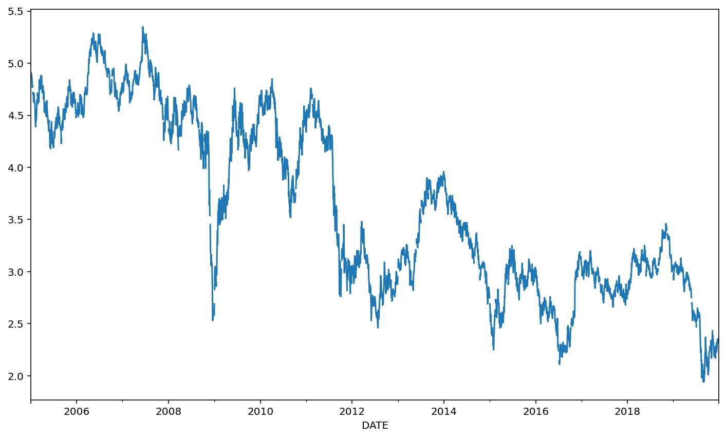
Look at the x-axis! It’s automatically labeled for us. Thanks, Python.
Let’s now plot the Treasury yield curve for ‘2016-06-07’. Recall that we can access the data like so:
ts.loc['2016-06-07', data_list]
DGS1MO    0.20
DGS3MO    0.28
DGS6MO    0.43
DGS1      0.59
DGS2      0.78
DGS5      1.23
DGS7      1.51
DGS10     1.72
DGS30     2.54
Name: 2016-06-07 00:00:00, dtype: float64
The maturity times for these securities are:
mat = [1, 3, 6, 12, 24, 60, 84, 120, 360]
We can then plot the yield curve using seaborn.
import seaborn as sns
sns.lineplot(x=mat, y=ts.loc['2016-06-07', data_list])
<AxesSubplot:ylabel='2016-06-07 00:00:00'>
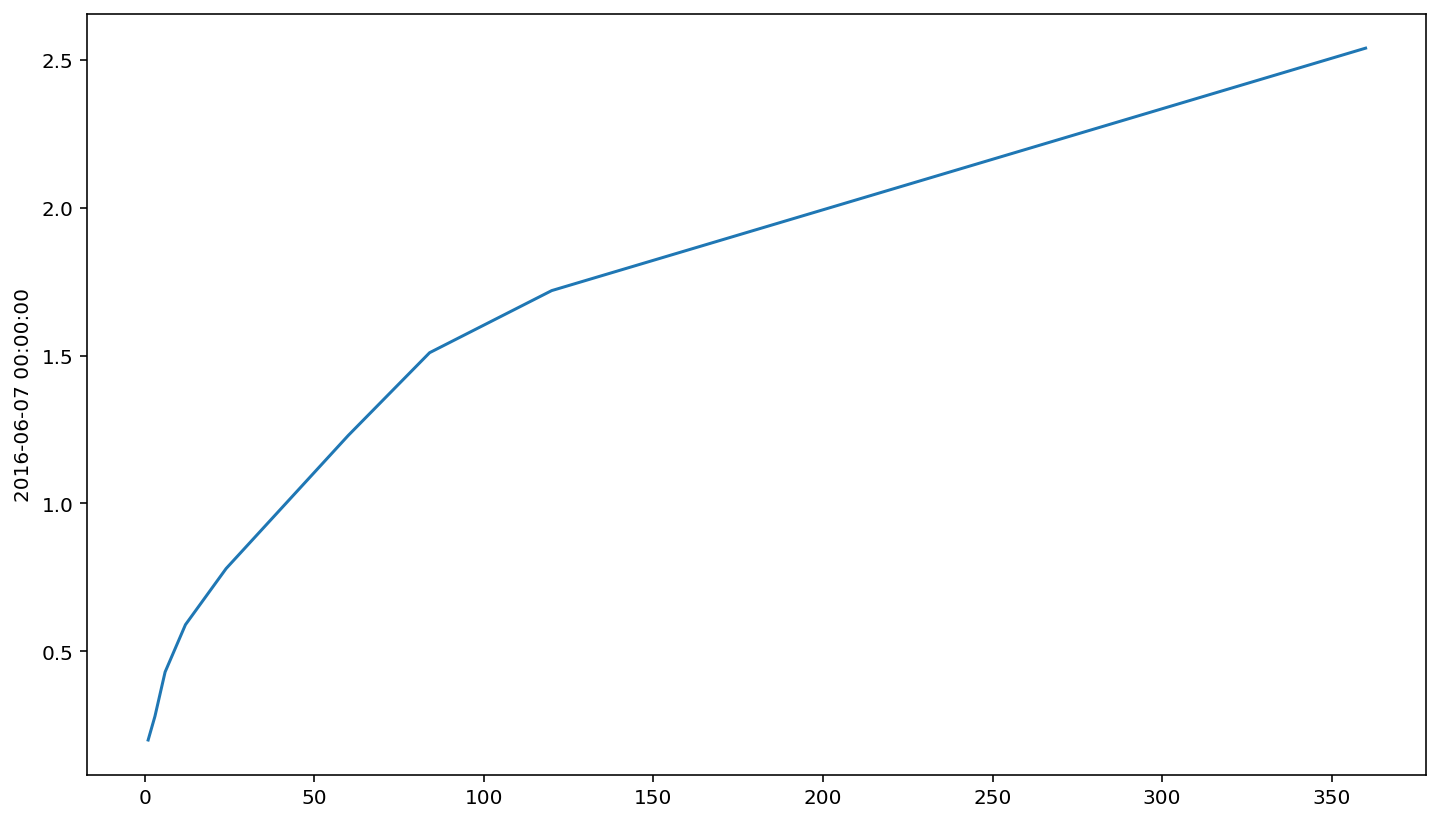
The yield curve does not always have this shape to it, though what’s shown above is the “standard” appearance. Typically, the yield curve is upward-sloping and somewhat curvy.
In contrast, the yield curve may sometimes invert. That is, it will have places in the curve that are downward-sloping.
sns.lineplot(x=mat, y=ts.loc['2007-01-02', data_list])
<AxesSubplot:ylabel='2007-01-02 00:00:00'>
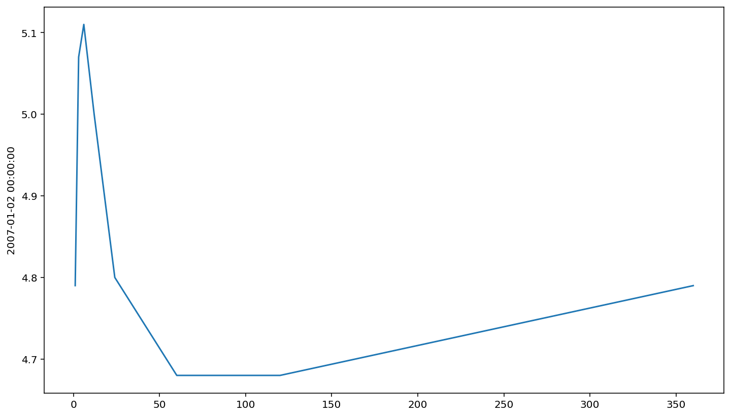
The usual place where we look for this is in the 10-year Treasury minus the 2-year Treasury.
ts['Slope'] = ts['DGS10'] - ts['DGS2']
ts['Slope'].plot()
<AxesSubplot:xlabel='DATE'>
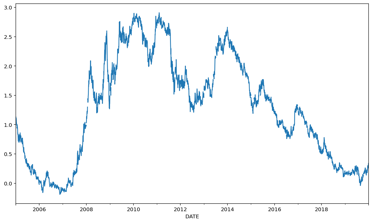
When this slope (the difference between the 10 year and 2 year) is negative, we refer to this as a yield curve inversion.
These inversion events are reasonably good predictors of recessions.
Let’s test this idea. Begin by getting a series of data about when recessions occur from FRED.
recession = web.DataReader('JHDUSRGDPBR', 'fred', start, end)
recession.head()
| JHDUSRGDPBR | |
|---|---|
| DATE | |
| 2005-01-01 | 0.0 |
| 2005-04-01 | 0.0 |
| 2005-07-01 | 0.0 |
| 2005-10-01 | 0.0 |
| 2006-01-01 | 0.0 |
The data series 'JHDUSRGDPBR' is a list of recessions. The value will be 1 when there is a recession and 0 when there is not a recession.
Let’s now merge the recession data. Note that the recession data is observed once per quarter. We should convert all data to a quarterly frequency before preceeding.
tsq = ts.to_period('Q')
tsq.head()
| DGS1MO | DGS3MO | DGS6MO | DGS1 | DGS2 | DGS5 | DGS7 | DGS10 | DGS30 | DGS30 growth | Slope | |
|---|---|---|---|---|---|---|---|---|---|---|---|
| DATE | |||||||||||
| 2005Q1 | 1.99 | 2.32 | 2.63 | 2.79 | 3.10 | 3.64 | 3.94 | 4.23 | 4.85 | NaN | 1.13 |
| 2005Q1 | 2.05 | 2.33 | 2.63 | 2.82 | 3.20 | 3.72 | 4.02 | 4.29 | 4.91 | 0.012371 | 1.09 |
| 2005Q1 | 2.04 | 2.33 | 2.63 | 2.83 | 3.22 | 3.73 | 4.02 | 4.29 | 4.88 | -0.006110 | 1.07 |
| 2005Q1 | 2.04 | 2.31 | 2.63 | 2.82 | 3.18 | 3.71 | 4.01 | 4.29 | 4.89 | 0.002049 | 1.11 |
| 2005Q1 | 2.03 | 2.32 | 2.63 | 2.82 | 3.20 | 3.73 | 4.03 | 4.29 | 4.88 | -0.002045 | 1.09 |
recession = recession.to_period('Q')
recession.head()
| JHDUSRGDPBR | |
|---|---|
| DATE | |
| 2005Q1 | 0.0 |
| 2005Q2 | 0.0 |
| 2005Q3 | 0.0 |
| 2005Q4 | 0.0 |
| 2006Q1 | 0.0 |
Note that the term structure data has multiple observations for a given quarter. Suppose that we only want to use the first observation. That is, at the start of a quarter, what does the term structure look like? We can remove duplicate index values to get rid of the observations that do not correspond to the first observation for each quarter using .duplicated().
tsq = tsq[~tsq.index.duplicated(keep='first')]
tsq.head()
| DGS1MO | DGS3MO | DGS6MO | DGS1 | DGS2 | DGS5 | DGS7 | DGS10 | DGS30 | DGS30 growth | Slope | |
|---|---|---|---|---|---|---|---|---|---|---|---|
| DATE | |||||||||||
| 2005Q1 | 1.99 | 2.32 | 2.63 | 2.79 | 3.10 | 3.64 | 3.94 | 4.23 | 4.85 | NaN | 1.13 |
| 2005Q2 | 2.66 | 2.80 | 3.13 | 3.34 | 3.75 | 4.13 | 4.29 | 4.46 | 4.72 | -0.008403 | 0.71 |
| 2005Q3 | 3.02 | 3.17 | 3.38 | 3.51 | 3.76 | 3.84 | 3.92 | 4.06 | 4.28 | 0.021480 | 0.30 |
| 2005Q4 | 3.22 | 3.61 | 4.02 | 4.09 | 4.21 | 4.25 | 4.31 | 4.39 | 4.58 | 0.011038 | 0.18 |
| 2006Q1 | NaN | NaN | NaN | NaN | NaN | NaN | NaN | NaN | NaN | NaN | NaN |
The observation at '2006Q1' is troubling. Why is there missing data there?
ts.loc['2005-12-29':'2006-01-03']
| DGS1MO | DGS3MO | DGS6MO | DGS1 | DGS2 | DGS5 | DGS7 | DGS10 | DGS30 | DGS30 growth | Slope | |
|---|---|---|---|---|---|---|---|---|---|---|---|
| DATE | |||||||||||
| 2005-12-29 | 3.67 | 4.01 | 4.34 | 4.35 | 4.38 | 4.33 | 4.34 | 4.37 | 4.49 | -0.004435 | -0.01 |
| 2005-12-30 | 4.01 | 4.08 | 4.37 | 4.38 | 4.41 | 4.35 | 4.36 | 4.39 | 4.51 | 0.004454 | -0.02 |
| 2006-01-02 | NaN | NaN | NaN | NaN | NaN | NaN | NaN | NaN | NaN | NaN | NaN |
| 2006-01-03 | 4.05 | 4.16 | 4.40 | 4.38 | 4.34 | 4.30 | 4.32 | 4.37 | 4.52 | NaN | 0.03 |
It’s unclear why the first observation for the first quarter of 2006 is missing, but we don’t want to lose that quarter of data simply because one date has missing data. Let’s fill in the data. The method we’ll use to do so is 'ffill', which stands for forward fill. Pandas will take the most recent data (in this case '2005-12-30') and use that to fill in the missing data (at '2006-01-02').
ts = ts.fillna(method='ffill')

ts.loc['2005-12-29':'2006-01-03']
| DGS1MO | DGS3MO | DGS6MO | DGS1 | DGS2 | DGS5 | DGS7 | DGS10 | DGS30 | DGS30 growth | Slope | |
|---|---|---|---|---|---|---|---|---|---|---|---|
| DATE | |||||||||||
| 2005-12-29 | 3.67 | 4.01 | 4.34 | 4.35 | 4.38 | 4.33 | 4.34 | 4.37 | 4.49 | -0.004435 | -0.01 |
| 2005-12-30 | 4.01 | 4.08 | 4.37 | 4.38 | 4.41 | 4.35 | 4.36 | 4.39 | 4.51 | 0.004454 | -0.02 |
| 2006-01-02 | 4.01 | 4.08 | 4.37 | 4.38 | 4.41 | 4.35 | 4.36 | 4.39 | 4.51 | 0.004454 | -0.02 |
| 2006-01-03 | 4.05 | 4.16 | 4.40 | 4.38 | 4.34 | 4.30 | 4.32 | 4.37 | 4.52 | 0.004454 | 0.03 |
With that data problem fixed, we can go back to the quarterly data. Let’s re-make the quarterly information.
tsq = ts.to_period('Q')
tsq = tsq[~tsq.index.duplicated(keep='first')]
tsq.head()
| DGS1MO | DGS3MO | DGS6MO | DGS1 | DGS2 | DGS5 | DGS7 | DGS10 | DGS30 | DGS30 growth | Slope | |
|---|---|---|---|---|---|---|---|---|---|---|---|
| DATE | |||||||||||
| 2005Q1 | 1.99 | 2.32 | 2.63 | 2.79 | 3.10 | 3.64 | 3.94 | 4.23 | 4.85 | NaN | 1.13 |
| 2005Q2 | 2.66 | 2.80 | 3.13 | 3.34 | 3.75 | 4.13 | 4.29 | 4.46 | 4.72 | -0.008403 | 0.71 |
| 2005Q3 | 3.02 | 3.17 | 3.38 | 3.51 | 3.76 | 3.84 | 3.92 | 4.06 | 4.28 | 0.021480 | 0.30 |
| 2005Q4 | 3.22 | 3.61 | 4.02 | 4.09 | 4.21 | 4.25 | 4.31 | 4.39 | 4.58 | 0.011038 | 0.18 |
| 2006Q1 | 4.01 | 4.08 | 4.37 | 4.38 | 4.41 | 4.35 | 4.36 | 4.39 | 4.51 | 0.004454 | -0.02 |
Now we can merge the two quarterly DataFrames.
ts_recession = tsq.merge(recession, on='DATE')
ts_recession.head()
| DGS1MO | DGS3MO | DGS6MO | DGS1 | DGS2 | DGS5 | DGS7 | DGS10 | DGS30 | DGS30 growth | Slope | JHDUSRGDPBR | |
|---|---|---|---|---|---|---|---|---|---|---|---|---|
| DATE | ||||||||||||
| 2005Q1 | 1.99 | 2.32 | 2.63 | 2.79 | 3.10 | 3.64 | 3.94 | 4.23 | 4.85 | NaN | 1.13 | 0.0 |
| 2005Q2 | 2.66 | 2.80 | 3.13 | 3.34 | 3.75 | 4.13 | 4.29 | 4.46 | 4.72 | -0.008403 | 0.71 | 0.0 |
| 2005Q3 | 3.02 | 3.17 | 3.38 | 3.51 | 3.76 | 3.84 | 3.92 | 4.06 | 4.28 | 0.021480 | 0.30 | 0.0 |
| 2005Q4 | 3.22 | 3.61 | 4.02 | 4.09 | 4.21 | 4.25 | 4.31 | 4.39 | 4.58 | 0.011038 | 0.18 | 0.0 |
| 2006Q1 | 4.01 | 4.08 | 4.37 | 4.38 | 4.41 | 4.35 | 4.36 | 4.39 | 4.51 | 0.004454 | -0.02 | 0.0 |
And finally, we can try to see if recessions are more likely when the slope is negative. In order to say that yield curve inversions might predict recessions, we need to use data from before a recession begins. For instance, does an inversion at quarter 3 of year \(t\) imply that a recession is likely to begin at quarter 4 of year \(t\)? We’ll use .shift() to make a lagged copy of the 'Slope' column.
ts_recession['Lagged Slope'] = ts_recession['Slope'].shift(1)
ts_recession.head()
| DGS1MO | DGS3MO | DGS6MO | DGS1 | DGS2 | DGS5 | DGS7 | DGS10 | DGS30 | DGS30 growth | Slope | JHDUSRGDPBR | Lagged Slope | |
|---|---|---|---|---|---|---|---|---|---|---|---|---|---|
| DATE | |||||||||||||
| 2005Q1 | 1.99 | 2.32 | 2.63 | 2.79 | 3.10 | 3.64 | 3.94 | 4.23 | 4.85 | NaN | 1.13 | 0.0 | NaN |
| 2005Q2 | 2.66 | 2.80 | 3.13 | 3.34 | 3.75 | 4.13 | 4.29 | 4.46 | 4.72 | -0.008403 | 0.71 | 0.0 | 1.13 |
| 2005Q3 | 3.02 | 3.17 | 3.38 | 3.51 | 3.76 | 3.84 | 3.92 | 4.06 | 4.28 | 0.021480 | 0.30 | 0.0 | 0.71 |
| 2005Q4 | 3.22 | 3.61 | 4.02 | 4.09 | 4.21 | 4.25 | 4.31 | 4.39 | 4.58 | 0.011038 | 0.18 | 0.0 | 0.30 |
| 2006Q1 | 4.01 | 4.08 | 4.37 | 4.38 | 4.41 | 4.35 | 4.36 | 4.39 | 4.51 | 0.004454 | -0.02 | 0.0 | 0.18 |
One last data-cleaning issue: statsmodels hates missing values. It throws a fit and stops working when it sees them. Notice that the first value of 'Lagged Slope' is missing, because we can’t observe a lag for the first data point.
To get rid of it, we use .dropna() to find all observations where the data is not missing.
ts_recession = ts_recession.dropna()
ts_recession.head()
| DGS1MO | DGS3MO | DGS6MO | DGS1 | DGS2 | DGS5 | DGS7 | DGS10 | DGS30 | DGS30 growth | Slope | JHDUSRGDPBR | Lagged Slope | |
|---|---|---|---|---|---|---|---|---|---|---|---|---|---|
| DATE | |||||||||||||
| 2005Q2 | 2.66 | 2.80 | 3.13 | 3.34 | 3.75 | 4.13 | 4.29 | 4.46 | 4.72 | -0.008403 | 0.71 | 0.0 | 1.13 |
| 2005Q3 | 3.02 | 3.17 | 3.38 | 3.51 | 3.76 | 3.84 | 3.92 | 4.06 | 4.28 | 0.021480 | 0.30 | 0.0 | 0.71 |
| 2005Q4 | 3.22 | 3.61 | 4.02 | 4.09 | 4.21 | 4.25 | 4.31 | 4.39 | 4.58 | 0.011038 | 0.18 | 0.0 | 0.30 |
| 2006Q1 | 4.01 | 4.08 | 4.37 | 4.38 | 4.41 | 4.35 | 4.36 | 4.39 | 4.51 | 0.004454 | -0.02 | 0.0 | 0.18 |
| 2006Q2 | 4.66 | 4.67 | 4.86 | 4.86 | 4.86 | 4.85 | 4.86 | 4.88 | 4.90 | 0.000000 | 0.02 | 0.0 | -0.02 |
Now, we can use statsmodels to run a logistic regression (since the y variable, 'JHDUSRGDPBR' is only ever 0 or 1).
One tricky element here is that the name for our \(x\) variable is 'Lagged Slope'. Python will get confused by this; if we write 'JHDUSRGDPBR ~ Lagged Slope' then Python will parse this as a function
$\(
\text{JHDUSRGDPBR} = \beta_0 + \beta_1\text{Lagged} + \beta_2\text{Slope} + u
\)$
which is not what we want. To ensure that Python reads 'Lagged Slope' as one column name, use the Q() function. That is, refer to the variable as Q("Lagged Slope").
import statsmodels.formula.api as smf

model = smf.logit('JHDUSRGDPBR ~ Q("Lagged Slope")', data=ts_recession).fit()
print(model.summary())
Optimization terminated successfully.
         Current function value: 0.363198
         Iterations 6
                           Logit Regression Results
==============================================================================
Dep. Variable:            JHDUSRGDPBR   No. Observations:                   59
Model:                          Logit   Df Residuals:                       57
Method:                           MLE   Df Model:                            1
Date:                Sun, 26 Sep 2021   Pseudo R-squ.:                0.002790
Time:                        21:01:12   Log-Likelihood:                -21.429
converged:                       True   LL-Null:                       -21.489
Covariance Type:            nonrobust   LLR p-value:                    0.7291
=====================================================================================
                        coef    std err          z      P>|z|      [0.025      0.975]
-------------------------------------------------------------------------------------
Intercept            -1.8067      0.685     -2.637      0.008      -3.150      -0.464
Q("Lagged Slope")    -0.1601      0.464     -0.345      0.730      -1.069       0.749
=====================================================================================
Negative \(\beta\) coefficients in a Logit model mean that the covariate (the right hand side variable) corresponding to that \(\beta\) coefficient are negatively predictive of the event. The “event” is an instance of y=1. So, what we see here is that a higher slope is negatively predictive of a recession.
If you load a much longer dataset, you can see a similar pattern over time.
The question is, why does this work? What’s the connection between the yield curve and recessions?
Let’s turn our attention to the expectations hypothesis, which is covered in earlier courses. Define \(y_t^{(i)}\) to be the one period interest rate at time \(t\) for a Treasury security with \(i\) periods to maturity. We thus have $\( \Big(1+y_t^{(2)}\Big)^2 = \Big(1+y_t^{(1)}\Big)\text{E}_t\Big[\Big(1+y_{t+1}^{(1)}\Big)\Big] \)$
That is, the cumulative return for holding a two-year Treasury to maturity should be the same return as holding a one-year Treasury to maturity and then holding another (future) one-year Treasury to maturity after that. At year \(t\), we don’t know what the one-year Treasury will be at in year \(t+1\). Thus, we say that the expected value of it is \(\text{E}_t\Big[\Big(1+y_{t+1}^{(1)}\Big)\Big]\), where \(\text{E}\) stands for expected value.
Let’s define the one-year forward rate as $\( \Big(1+f_{t}^{(1)}\Big) = \frac{\Big(1+y_t^{(2)}\Big)^2}{\Big(1+y_t^{(1)}\Big)} \)$
The value for \(f_{t}^{(1)}\) is something that we can calculate given other data at time \(t\). The Expectations Hypothesis says that this value should be a good estimate for the expected future spot rate, i.e.: $\( f_{t}^{(1)} = \text{E}_t\Big[1+y_{t+1}^{(1)}\Big] \)$
Compute the forward rate below.
tsq['1Y Forward'] = (1+tsq['DGS2'])**2/(1+tsq['DGS1']) - 1
tsq.head()
| DGS1MO | DGS3MO | DGS6MO | DGS1 | DGS2 | DGS5 | DGS7 | DGS10 | DGS30 | DGS30 growth | Slope | 1Y Forward | |
|---|---|---|---|---|---|---|---|---|---|---|---|---|
| DATE | ||||||||||||
| 2005Q1 | 1.99 | 2.32 | 2.63 | 2.79 | 3.10 | 3.64 | 3.94 | 4.23 | 4.85 | NaN | 1.13 | 3.435356 |
| 2005Q2 | 2.66 | 2.80 | 3.13 | 3.34 | 3.75 | 4.13 | 4.29 | 4.46 | 4.72 | -0.008403 | 0.71 | 4.198733 |
| 2005Q3 | 3.02 | 3.17 | 3.38 | 3.51 | 3.76 | 3.84 | 3.92 | 4.06 | 4.28 | 0.021480 | 0.30 | 4.023858 |
| 2005Q4 | 3.22 | 3.61 | 4.02 | 4.09 | 4.21 | 4.25 | 4.31 | 4.39 | 4.58 | 0.011038 | 0.18 | 4.332829 |
| 2006Q1 | 4.01 | 4.08 | 4.37 | 4.38 | 4.41 | 4.35 | 4.36 | 4.39 | 4.51 | 0.004454 | -0.02 | 4.440167 |
Now, we shift the data ahead by 4 periods so we get a one year lag.
tsq['Last Year 1Y Forward'] = tsq['1Y Forward'].shift(4)
tsq.head()
| DGS1MO | DGS3MO | DGS6MO | DGS1 | DGS2 | DGS5 | DGS7 | DGS10 | DGS30 | DGS30 growth | Slope | 1Y Forward | Last Year 1Y Forward | |
|---|---|---|---|---|---|---|---|---|---|---|---|---|---|
| DATE | |||||||||||||
| 2005Q1 | 1.99 | 2.32 | 2.63 | 2.79 | 3.10 | 3.64 | 3.94 | 4.23 | 4.85 | NaN | 1.13 | 3.435356 | NaN |
| 2005Q2 | 2.66 | 2.80 | 3.13 | 3.34 | 3.75 | 4.13 | 4.29 | 4.46 | 4.72 | -0.008403 | 0.71 | 4.198733 | NaN |
| 2005Q3 | 3.02 | 3.17 | 3.38 | 3.51 | 3.76 | 3.84 | 3.92 | 4.06 | 4.28 | 0.021480 | 0.30 | 4.023858 | NaN |
| 2005Q4 | 3.22 | 3.61 | 4.02 | 4.09 | 4.21 | 4.25 | 4.31 | 4.39 | 4.58 | 0.011038 | 0.18 | 4.332829 | NaN |
| 2006Q1 | 4.01 | 4.08 | 4.37 | 4.38 | 4.41 | 4.35 | 4.36 | 4.39 | 4.51 | 0.004454 | -0.02 | 4.440167 | 3.435356 |
The Expectations Hypothesis says that this one year old forward rate should be the same, on average, as what the spot rate is. We can test this with linear regression.
tsq2 = tsq.dropna().copy()

eh = smf.ols('DGS1 ~ Q("Last Year 1Y Forward")', data=tsq2).fit()

print(eh.summary())
                            OLS Regression Results
==============================================================================
Dep. Variable:                   DGS1   R-squared:                       0.686
Model:                            OLS   Adj. R-squared:                  0.680
Method:                 Least Squares   F-statistic:                     118.1
Date:                Sun, 26 Sep 2021   Prob (F-statistic):           3.34e-15
Time:                        21:07:09   Log-Likelihood:                -73.610
No. Observations:                  56   AIC:                             151.2
Df Residuals:                      54   BIC:                             155.3
Df Model:                           1
Covariance Type:            nonrobust
=============================================================================================
                                coef    std err          t      P>|t|      [0.025      0.975]
---------------------------------------------------------------------------------------------
Intercept                    -0.4118      0.207     -1.985      0.052      -0.828       0.004
Q("Last Year 1Y Forward")     0.9291      0.086     10.865      0.000       0.758       1.101
==============================================================================
Omnibus:                        0.288   Durbin-Watson:                   0.273
Prob(Omnibus):                  0.866   Jarque-Bera (JB):                0.464
Skew:                          -0.118   Prob(JB):                        0.793
Kurtosis:                       2.622   Cond. No.                         4.58
==============================================================================

Notes:
[1] Standard Errors assume that the covariance matrix of the errors is correctly specified.
The \(\beta\) coefficient is close to 1, which is expected given the predicted relationship.
What can the Expectations Hypothesis tell us? Well, if there is a yield curve inversion, it’s because the market is expecting interest rates to be lower in the future than they are today. Why would the market expect that? Well, during recessions, the Fed will lower rates to stimulate growth. Thus, it’s pretty natural, when you think about it, to expect an inversion to occur before a recession. All it means is that bond traders are, on average, expecting a recession to occur. A more pertinent question is why bond traders see a recession coming. We’d need more data to answer that question.